=VLOOKUP(One Function to Rule Them All...)
- Aug 24, 2015
- 3 min read

Microsoft Excel has a very powerful function that helps users combine data from multiple sources into one table in a spreadsheet.
For example, if you have January’s budgeted sales data in one tab of a spreadsheet and the January’s actual sales data in a separate tab on the same spreadsheet or a different spreadsheet, it would be cumbersome to analyze the budgeted vs actual sales data. It will be much easier if both sets of data are on the same tab. If we can combine data from multiple spreadsheets into one spreadsheet, we can save hours of time and reduce data entry errors dramatically. VLOOKUP is the perfect solution for such scenarios.
VLOOKUP (vertical lookup) function allows user to look for a specific value in one column of data inside a table, and then fetch a value from another column in the same row. It can also return the closest match to the value being looked up so that each row in the table can represent ranges of values. The table being looked into can be within a different spreadsheet to the one currently being worked on, and this spreadsheet can be shared between multiple users.
This makes VLOOKUP unquestionably one of the most useful power-function of Excel. Learning VLOOKUP formula will change your basic approach towards data forever.
VLOOKUP in Action
Here I will take you through a tutorial on how to use VLOOKUP function.

You will see the first tab; “Sales by Employee” has Quarter-1 revenue information by individual Employee IDs and the second tab; “Employee Detail” has information about each employee following their unique Employee ID.
In this example, Sales by Employee tab is difficult to analyze just by the Employee ID. It would have been helpful if we can see the name of the employee, the region he/she belongs to, and his/her employment status. Here, we will use VLOOKUP to fetch the related information from the pool of data in the second tab, Employee Detail.
1. On the Sales by Employee tab, add three columns for employee name, region, and status.
2. Select cell C2 to insert the VLOOKUP function
3. There are several ways you can add a formula into a cell. You can manually type the function (=VLOOKUP), add it from the formula tab on the ribbon, or click on the formula bar fx sign beside the formula bar.

4. After opening the Functions Arguments dialog box, you have to fill out four pieces of information. The function panel may seem intimidating with the terms, but it is simpler than it looks.

Lookup_value: The value you want to look up. The value you want to look up must be in the first column of the range of cells you specify in table-array.
Table_array: The range of cells in which the VLOOKUP will search for thelookup_value and the return value. The first column in the cell range must contain thelookup_value.
Col_index_num: the column number in the table_array argument from which the matching value must be returned. (Starting with 1 for the left-most column oftable-array)
Range_lookup: this is optional. A logical value that specifies whether you want to find exact match (False) or an approximate match (True). For this example, false must be used since we are dealing with employee data.
Define the Values
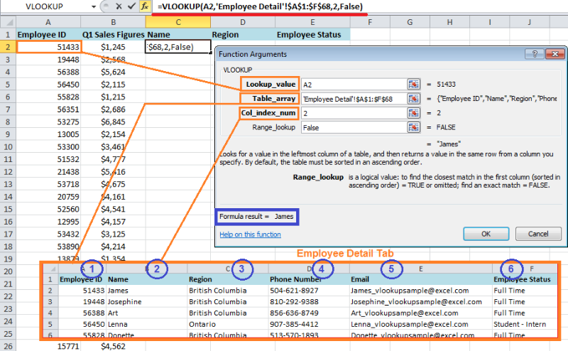
For the illustration purposes, I have overlaid the Employee Detail tab to show the relationships.

Lookup_value: This is your starting point. In this example, type or click on A2. Here, you are requesting excel to select the value of cell A2, which is the Employee ID “51433”.
Table_array: This is a range for your lookup table. The range can be on your existing worksheet or another worksheet. Here using absolute ($) is recommended since, we will be dragging the formulas down. Just simply go to the Employee Detail tab and select the range and hit F4 to make the range absolute.
Col_index_num: This is the number of the column on the lookup table that has the information you need. In our example, we want column #2 because we are looking for Employee name.
Range_lookup: This field defines how close a match should exist between your lookup value (A2) and the value in the leftmost column on the lookup table. In our example, we want an exact match so we will use “False.”
After filling out all four function arguments, you will be able to see the formula results on the bottom left corner of the function arguments(blue square box in the illustration).
After clicking OK, you will be able to see the results we were looking for. Now, you can simply drag the formula down to the bottom of the table.
Now you know how to use the VLOOKUP, you can try filling out the region and employee status columns with VLOOKUP.


Comments